Create Random Numbers in Excel: 5 Easy Ways

If you want to create random numbers in Excel, you can use the RAND and RANDBETWEEN functions.

Meanwhile, Office 365 users can use the RANDARRAY function to create random numbers from a group of data in a certain range of cells.

So, in this guide, I’ll give several examples of how to create random numbers in Excel using the RAND, RANDBETWEEN, and RANDARRAY functions.

To help you practice generating random numbers in Excel, please download the following Excel file:

Create Random Numbers in Excel with the RAND Function (Decimal numbers 0 to 1)

The RAND function in Excel can help you create random numbers in decimals from 0 to 1 such as 0.1, 0.25, 0.4457, etc.

For example, I want to create random numbers in Excel in cells A1 to A10. Pay attention to the following stages:

1. Type the RAND function in cell A1 as follows: =RAND().
2. Perform Excel Autofill (Click-Hold-Drag) to create random numbers in cells A2 to A10. Here are the results:

For a deeper understanding, let’s look at the details of the RAND formula above:

RAND Excel Formula Breakdown:
=RAND()

Explanation:
Create a Random Number (decimal) from 0 – 1 That Doesn’t Exist in This Excel File

Note: All random numbers will change if there are any changes to this Workbook.

To anticipate that the random numbers will not change, please copy all these Random Numbers and use Paste Values as follows:

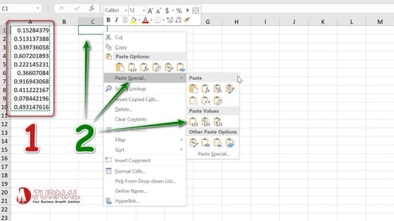
1. Select the cell range A1:A10, then press the Ctrl + C keys on the keyboard simultaneously.
2. Right-click on cell C1 and click Paste Special. Then select Value. Here are the results:

You can copy the random numbers in the cell range C1:C10 and use them as you wish. Then, if necessary, you can delete Random Numbers in the range A1:A10.

Trick: Modify the RAND Function

In other examples, you may need to modify the RAND Function. For example, if you want to generate a random decimal number from 50 to 60, please follow these steps:

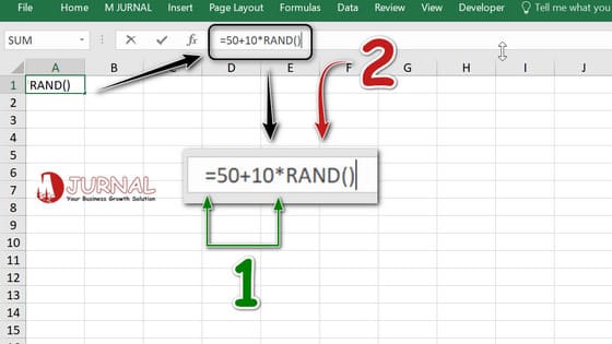
1. Type =50+10* in cell A1
2. Enter the RAND function so that the formula becomes =50+10*RAND() and here are the results:

You can see, Excel returns a random number between 50 and 60. The key is 50+60*. Here’s the explanation:

Breakdown of the Modified RAND Formula in Excel:
=50+10*RAND()

Explanation:
50 plus 10 times a Random Numbers (decimal) from 0 to 1

Create Random Numbers in Excel Using Integers

You can use the RANDBETWEEN function to create random numbers in Excel between 2 integers (negative or positive).

For example, to create random numbers from -5 to 20 in the range C1:C10, please follow these steps:

1. Type the RANDBETWEEN function in cell C1 as follows: =RANDBETWEEN(.
2. Enter the smallest number (in this example -5).
3. Type the formula separation operator – comma (,). So the function becomes =RANDBETWEEN(-5,
4. Enter the largest number (in this example it is 20). Then type the closing bracket “)” and press Enter. Here are the results:

Note: You can do Excel Autofill or copy-paste to create random numbers in other cells.

Next, let’s pay attention to the breakdown of the RANDBETWEEN function used:

RANDBETWEEN Excel Formula Breakdown:
=RAND(-5,20)

Explanation:
Create Random Numbers (integers) that are not in this Excel file, from -5 to 20

Just like the RAND function, to use this random number, please copy-paste the value of the random number generated by the RANDBETWEEN function.

Create Random Numbers in Excel Using the RANDARRAY Function

The RANDARRAY function can also be called a combination of the RAND and RANDBETWEEN functions in Excel. However, unfortunately, the RANDARRAY function can only be used by Office 365 users.

If this functionality is what you need, you can always upgrade your subscription to Office 365.

However, before thinking about upgrading the service, it’s a good idea to first know what you get from the RANDARRAY function in Excel.

Let’s study the following examples…

#1 – RANDARRAY for Random Decimal Numbers

By default, the RANDARRAY function will provide a random decimal number from 0 to 1. This is the same as the RAND function.

The difference is that you can generate random numbers in 2 or more cells at once.

For example, I want to generate random numbers (decimal) in the range A1:B5 using the RANDARRAY Function. Pay attention to the following steps:

1. Type the RANDARRAY function in cell A1 as follows: =RANDARRAY(
2. Enter the number of rows, namely 5, then type the formula separation operator – comma “,”.
3. Enter the number of columns, namely 2, then type the closing bracket “)” and press Enter. The result is like the image above.

Excel automatically creates random decimal numbers in cells A1 through B5.

Again… Let’s learn the meaning of the RANDARRAY function used.

RANDARRAY Excel Formula Breakdown:
=RANDARRAY(5,2)

Explanation:
Create Random Decimal Numbers in an Array: 5 rows and 2 columns, which are not in this Excel file.

You just need to enter the RANDARRAY Function in cell A1. Then, arguments 5 and 2 will calculate the number of rows and number of columns (this is used in the ARRAY function).

#2 – RANDARRAY for Random Integer Numbers

You can also use the RANDARRAY function in Office 365 to generate random integer numbers.

For example, I want to generate random integer numbers from 20 to 80. Then display them in 10 rows and 1 column. Please follow the following steps:

1. Type the RANDARRAY function in cell A1 as follows: =RANDARRAY(.
2. Enter the number of rows, namely 10. Then type the formula separator operator – comma “,”.
3. Enter the number of columns, namely 1. Then type the formula separator operator – comma “,”.
4. Type the lowest number. In this example it is 20, then separate the formula arguments with commas “,”
5. Type the highest number. In this example it is 80, then separate the formula arguments with a comma “,”.
6. Select or type TRUE and close the bracket “)”. So the function becomes =RANDARRAY(10,1,20,80,TRUE).

Now, let me explain the breakdown of the RANDARRAY function used:

RANDARRAY Excel Formula Breakdown:
=RANDARRAY(10,1,20,80,TRUE)

RANDARRAY Excel Formula Breakdown:
Create Random Numbers in an Array: 10 rows and 1 column, with criteria: Smallest Number = 20 and Largest Number = 80. Give Integer results

With these 5 arguments, Excel will return a random number from 20 to 80 which is an integer. Then returns the results in the specified 10 rows and 1 column.

Same as RAND and RANDBETWEEN Functions. You must copy the results of the RANDARRAY function by pasting the values so that these results do not change.

BONUS: Random Data Alternative in Excel

In certain circumstances, you may want to randomize data in the form of numbers, text such as names, or dates.

I also wrote a guide on how to randomize data order using a combination of the RAND function and Excel’s Sort & Filter feature (currently only available in Indonesian).

Apart from that, you can also use a combination of the INDEX, RANDBETWEEN, and COUNTA functions to retrieve data randomly from the data list.

For example, to randomly determine the name of the lottery winner as shown in the following image:

In this example, I use the formula =INDEX(A2:A11,RANDBETWEEN(1,COUNTA(A2:A11))), then Excel can randomize the names of the lottery winners.

In conclusion:

There are many ways to generate random numbers in Excel. You can use the RAND function to create random decimal numbers or use the RANDBETWEEN function to create random integers.

If these two functions don’t suit your needs, use the RANDARRAY function in Office 365 for great flexibility.

Lastly, not only to generate random numbers, you can also randomize a list of names for a specific purpose – like a lottery.

Apart from that, what you need to understand is the function syntax in Excel. Understand syntax, meaning you have to understand the meaning of each argument in the formula and how to write it.

Next, not just have a guide about creating random numbers in Excel, I have various other guides about Excel.

Please learn more through the following guide shortcuts: